Realization of Amplitude Modulation using MATLAB.

Objective:

• To study and learn the amplitude modulation.
• To learn the MATLAB coding for amplitude modulation.
• To observe the amplitude modulation wave form.

Theory:

The amplitude modulation is a process in which the amplitude of carrier c(t) is varied about a mean value with the massage signal m(t). Amplitude modulation (AM) is the family of modulation schemes in which the amplitude of a sinusoidal carrier is changed as a function of the modulating message signal.

Let, the massage signal is, m(t)= A_mcos (2 πf_mt)

And the carrier signal is, c(t)= A_ccos(2πf_ct)

So the modulated signal is,

 s(t)= A_c cos(2πf_ct)+ A_m cos(2πf_mt)

      = A_c (1+k_a m(t))sin(2πf_ct)

Here A_c  and A_m  is the amplitude of carrier and message signal f_c and f_m  is the frequency of carrier and message signal and k_a is a constant called the amplitude sensitivity of the modulated signal.

If kam(t)<1 and fc>>ωm  then modulation will be perfect. In amplitude modulation only the amplitude of the carrier wave is changed in accordance the signal. However the frequency of the modulated wave remains the same.

Require instrument:

1.    Mat lab software

2.     Computer

MATLAB code:

Fc= input('Carrier signal Frequency=');

Fm=input('Message Signal Frequency=');

Ac=input('Carrier signal Amplitude=');

Am=input('Message Signal Amplitude=');

t=0:0.1:100;

A=2*pi*Fc*t;

Ct=Ac*cos(A);

subplot(3,1,1);

plot(t,Ct,'r')

xlabel('Time');

ylabel('Amplitude');

title('Carrier Signal');

grid on;

B=2*pi*Fm*t;

Mt=Am*cos(B);

subplot(3,1,2);

plot(t,Mt,'g')

xlabel('Time');

ylabel('Amplitude');

title('Message Signal');

grid on;

M=Fm/Fc;

Mod=M*Mt.*Ct;

AM=Ct+Mod;

subplot(3,1,3);

plot(t,AM,'b')

xlabel('Time');

ylabel('Amplitude');

title('Amplitude Modulated Signal');

grid on;

Simulation Result:

Figure 01: The Carrier Signal, Message Signal and Amplitude Modulated Signal.

Discussion:

1.     The carrier frequency fc  is much greater than the message frequency fm .

2.     The amplitude of the carrier and message signal should take the same value.

3.     It can send massage without interference.

4.     The condition  kam(t)<1  should be satisfied.

Conclusion:

Amplitude modulated signals are generated by multiplying message signals with a carrier and adding the carrier to this product. The amplitude of the message signal is varied to produce different values of the modulation index. The MATLAB environment can be an effective tool for viewing the effects of various forms of modulation.

Some Important MATLAB codes for Control Theory

We can solve some kinds of Analysis of Control system using MATLAB codes. Control Systems Engineering is an exciting and challenging field and is a multidisciplinary subject. Control systems in an interdisciplinary field covering many areas of engineering and sciences. Control systems exist in many systems of engineering, sciences, and in human body. Some type of control systems affects most aspects of our day-to-day activities.

If H(s)=(x3-6x2+3x+14)/(x5+x4-5x3-9x2+x-11) is obtain the partial-fraction expansion of the ratio of two polynomials then we can determine the zero & pole by using MATLAB code.

MATLAB CODE:

                                        numerator=[1,-6,3,14]

                                       denominator=[1,1,-5,-9,1,-11]

                                       [zero,pole]=tf2zp(numerator,denominator)

Output of the code:    

                                       numerator =1    -6     3    14

                                      denominator = 1     1    -5    -9     1   -11

                                     zero =4.7466

                                               2.4549

                                              -1.2015

                                     pole =2.5483         

                                               -1.9958 + 0.9768i

                                               -1.9958 - 0.9768i

                                               0.2216 + 0.9084i

                                               0.2216 - 0.9084i

We can use the MATLAB command step (sys) may also be used to obtain the unit-step response, rise time, peak time, max overshoot & settling time of a system. If H(s)= (16x+10)/(5x3+11x2+19x+10) is a control system then the command  step (sys) can be used where the system is defined by  sys = tf (num, den). The following MATLAB step commands with left hand arguments are used then no plot is shown on the screen.

MATLAB CODE:

                         num = [0,0,16,10]

                         den = [5,11,19,10]

                         t = 0:0.2.5:10;

                         [x, y, t] =step(num, den, t);

                         plot(t, y)

                         title ('Plot of unit-step response curves')

                          xlabel ('t Sec')

                         ylabel ('Response')

                         grid on

                        r1 = 1; while y(r1) < 0.1, r1 = r1 + 1; end

                        r2 = 1; while y(r2) < 0.9, r2 = r2 + 1; end

                        rise time = (r2-r1)*0.02

                        [ymax, tp] = max(y);

                       peak time = (tp-1)*0.02

                      max overshoot = ymax-1

                       s = 1001; while y(s) > 0.98 & y(s) < 1.02; s = s-1; end

                       settling time = (s-1)*0.02

Output of the code:

                            

                            num =0     0    16    10

                            den = 5    11    19    10

                            rise time =0.7800

                            peak time =2.1400

                            max overshoot =0.4752

                           settling  time =7.4200

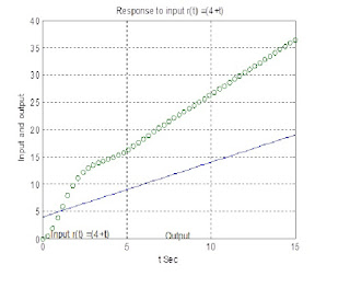
By using MATLAB codes we can also solve the Unit Step Response of the Control system.

MATLAB CODE: 

                                      num = [0 0 16 20];

                                     den = [5 11 16 10];

                                      t = 0:0.3:15;

                                      r1 = (4+t);

                                     y1 = lsim(num, den, r1,t);

                                      plot(t, r1,t, y1,'o')

                                     grid on

                                     title('Response to input r(t) =(4+t)')

                                     xlabel('t Sec')

                                     ylabel('Input and output')

                                    text(0.5, 0.9, 'Input r1 =(4+t)')

                                    text(7.3, 0.6, 'Output')

Output of the code:

                            

MATLAB codes can also be used for determining Root Locus, Bode diagram & Nyquist plot of a control system if  H(s)= (x+1)/(x3+3.6x2) is a control system.

MATLAB CODE: 

                            For Root Locus:   

                                                           num = [0 0 1 1];

                                                          den = [1 3.6 0 0];

                                                           K1 = 0:0.1:2;

                                                           K2 = 2:0.02:2.5;

                                                           K3 = 2.5:0.5:10;

                                                           K4 = 10:1:50;

                                                           K5 = 50:5:900;

                                                          K = [K1 K2 K3 K4 K5];

                                                          r = rlocus(num, den, K);

                                                          plot(r, 'o')

                                                          grid on

                                                         title('Root - locus plot of G(s)H(s)')

                                                         xlabel('Real axis')

                                                         ylabel('Imaginary axis')

                     For Bode diagram:

                                                    num = [0 0 10 10];

                                                    den = [1 3.6 0 0];

                                                    grid on

                                                    bode(num, den);

                                             title ('Bode diagram of G(s)H(s)')

                                

                       For Nyquist plot:

                                                 num = [0 0 10 10];

                                                 den = [1 3.6 0 0];

                                                 nyquist(num,den)

                                                 grid on

Output of the code:

                   

                     

                     

By using MATLAB code we can solve transfer function of a state space equation. Now here is the MATLAB code.

MATLAB CODE:

                                            syms s

                                            A = [1 0];

                                            B = [s+3 1;-2 s];

                                           C = [0; 1];

                                            A*inv(B)*C

Output of the code: 

                                          ans = -1/(s^2+3*s+2)

The Laplace transformation method is an operational method that can be used to find the transforms of time functions, the inverse Laplace transformation using the partial fraction expansion of H(s), where A(s). We present the computational methods with MATLAB to obtain the partial-fraction expansion of H(s) and the zeros and poles of H(s). MATLAB can be used to obtain the partial-fraction expansion of the ratio of two polynomials H(s)= B(s)/A(s). The coefficients of the numerator and denominator of B(s)/A(s) are specified by the num and den vectors. The MATLAB command r, p, k = residue(num, den) is used to determine the residues, direct terms of a partial-fraction expansion of the ratio of two polynomials B(s) and A(s) is then given by,

MATLAB CODE:

                                  num = [ 0 0 1 1 6];

                                  den = [1 1 1 0 12];

                                  [r, p, k] = residue(num, den)

                                 syms s

                                 f =((s*s)+s+6)/((s*s*s*s)+(s*s*s)+(s*s)+12);

                                 ilaplace(f)

Output of the code: 

                                  r =  0.0666 - 0.2011i

                                         0.0666 + 0.2011i

                                        -0.0666 - 0.2858i

                                        -0.0666 + 0.2858i

                                 p = -1.5069 + 1.4025i

                                       -1.5069 - 1.4025i

                                         1.0069 + 1.3482i

                                         1.0069 - 1.3482i

                                  k =[]

ans =      -1/9186*sum((245*_alpha^2+166*_alpha^3+291+1251*_alpha)*exp(_alpha*t),_alpha = RootOf(_Z^4+_Z^3+_Z^2+12))