We can
solve some kinds of Analysis of Control system using MATLAB codes. Control Systems Engineering is an
exciting and challenging field and is a multidisciplinary subject. Control systems in an
interdisciplinary field covering many areas of engineering and sciences.
Control systems exist in many systems of engineering, sciences, and in human
body. Some type of control systems affects most aspects of our day-to-day
activities.
If H(s)=(x 3 - 6 x 2 +3 x +14) /(x 5 + x 4 - 5 x 3 - 9 x 2 + x - 11)
MATLAB CODE:
numerator=[1,-6,3,14]
denominator=[1,1,-5,-9,1,-11]
[zero,pole]=tf2zp(numerator,denominator)
Output of the code:
numerator
=1 -6 3
14
denominator = 1 1
-5 -9 1
-11
zero =4.7466
2.4549
-1.2015
pole =2.5483
-1.9958 + 0.9768i
-1.9958 - 0.9768i
0.2216 + 0.9084i
0.2216 - 0.9084i
We
can use the MATLAB command step (sys) may also be used to obtain the unit-step
response, rise time, peak time, max overshoot & settling time of a system. If
H(s)= (16 x +10 )/(5 x 3 + 11 x 2 +19 x +10)
MATLAB CODE:
num = [0,0,16,10]
den = [5,11,19,10]
t = 0:0.2.5:10;
[x, y, t] =step(num,
den, t);
plot(t, y)
title ('Plot of
unit-step response curves')
xlabel ('t Sec')
ylabel ('Response')
grid on
r1 = 1; while y(r1)
< 0.1, r1 = r1 + 1; end
r2 = 1; while y(r2)
< 0.9, r2 = r2 + 1; end
rise time =
(r2-r1)*0.02
[ymax, tp] = max(y);
peak time = (tp-1)*0.02
max overshoot = ymax-1
s = 1001; while y(s)
> 0.98 & y(s) < 1.02; s = s-1; end
settling time = (s-1)*0.02
Output of the code:
num =0 0
16 10
den = 5 11
19 10
rise time =0.7800
peak time =2.1400
max overshoot =0.4752
settling time
=7.4200
By using
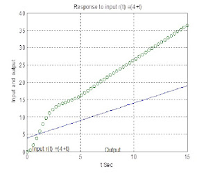
MATLAB codes we can also solve the Unit Step Response of the Control system.
MATLAB CODE:
num = [0
0 16 20];
den = [5
11 16 10];
t = 0:0.3:15;
r1 =
(4+t);
y1 =
lsim(num, den, r1,t);
plot(t,
r1,t, y1,'o')
grid on
title('Response to input r(t) =(4+t)')
xlabel('t
Sec')
ylabel('Input and output')
text(0.5,
0.9, 'Input r1 =(4+t)')
text(7.3,
0.6, 'Output')
Output of the code:
MATLAB
codes can also be used for determining Root Locus, Bode diagram & Nyquist
plot of a control system if H(s)= (x +1 )/(x 3 + 3.6 x 2)
MATLAB CODE:
For Root
Locus:
num = [0 0 1 1];
den = [1 3.6 0 0];
K1 = 0:0.1:2;
K2 = 2:0.02:2.5;
K3 = 2.5:0.5:10;
K4 = 10:1:50;
K5 = 50:5:900;
K = [K1
K2 K3 K4 K5];
r = rlocus(num, den, K);
plot(r, 'o')
grid on
title('Root - locus plot of G(s)H(s)')
xlabel('Real axis')
ylabel('Imaginary axis')
For Bode diagram:
num = [0 0 10 10];
den = [1 3.6 0 0];
grid on
bode(num, den);
title ('Bode diagram of G(s)H(s)')
For Nyquist plot:
num =
[0 0 10 10];
den =
[1 3.6 0 0];
nyquist(num,den)
grid on
Output of the code:
By using
MATLAB code we can solve transfer function of a state space equation. Now here
is the MATLAB code.
MATLAB CODE:
syms s
A =
[1 0];
B =
[s+3 1;-2 s];
C =
[0; 1];
A*inv(B)*C
Output of the code:
ans =
-1/(s^2+3*s+2)
The Laplace transformation method is an operational method
that can be used to find the transforms of time functions, the inverse Laplace
transformation using the partial fraction expansion of H(s), where A(s). We
present the computational methods with MATLAB to obtain the partial-fraction
expansion of H(s) and the zeros and poles of H(s). MATLAB can be used to obtain
the partial-fraction expansion of the ratio of two polynomials H(s)= B(s)/A(s).
The coefficients of the numerator and denominator of B(s)/A(s) are specified by
the num and den vectors. The MATLAB command r, p, k = residue(num, den) is used
to determine the residues, direct terms of a partial-fraction
expansion of the ratio of two polynomials B(s) and A(s) is then given by,
MATLAB
CODE:
num = [ 0 0 1
1 6];
den = [1 1 1
0 12];
[r, p, k] =
residue(num, den)
syms s
f
=((s*s)+s+6)/((s*s*s*s)+(s*s*s)+(s*s)+12);
ilaplace(f)
Output of the code:
r = 0.0666 - 0.2011i
0.0666
+ 0.2011i
-0.0666
- 0.2858i
-0.0666
+ 0.2858i
p = -1.5069 + 1.4025i
-1.5069
- 1.4025i
1.0069
+ 1.3482i
1.0069
- 1.3482i
k =[]
ans
=
-1/9186*sum((245*_alpha^2+166*_alpha^3+291+1251*_alpha)*exp(_alpha*t),_alpha
= RootOf(_Z^4+_Z^3+_Z^2+12))


Very informative post. Keep up the good work. I would really look forward to your other posts
ReplyDeletePanasonic - 13.1" Toughbook Notebook - 4 GB Memory - 500 GB Hard Drive
Panasonic - 15.4" Toughbook Notebook - 4 GB Memory and 256 GB Solid State Drive
This is useful to the students thank you for shared this..
Deletecan you please share how to solve the control systems problems by using SCILAB...